Quantum Computing (in development)
While in some movies the plot can get a bit ambitious and use the notion of quantum physics to introduce concepts such as time travel, teleportation and various magically working gadgets - that defy our everyday understanding of physics - it is also true that quantum physics, which deals with how things work at the atomic level, behaves in a different way than our intuition is used to.
Quantum computers are based on the principles of quantum physics, and although they will not help with the time-traveling part, they do possess some advantages over classical computers and are envisioned to help us solve problems that wouldn't be feasible with the current technology.
It's worth noting that a classical computer is a Turing machine, which means that it's theoretically capable of implementing any computer algorithm - even one that simulates a quantum computer - but this assumes that we have infinite time and memory at our disposal. So rather said, a quantum computer can help us solve tasks more efficiently than a classical computer, which could even mean that something that would require hundreds of years to perform classically can be reduced to a matter of minutes.
Classical Computing - in the Matrix Form
At a low level, in an ordinary computer, everything in the software part is made out of bits. A bit is the basic unit of information which represents two possible states. In a physical representation, some circuits can recognize a voltage lower than \(0.8V\) as one state, whereas the other possible state can be identified by a voltage higher than \(2.2V\).
In a computer representation, these two states are however simplified to \(0\) and \(1\). Fortunately for us, the bits are hidden by high-level routines which makes our life way easier, as it would be burdensome to manipulate them into performing a desired task.
However, to better contrast with what's to come, let's stick to the level of bits. We can represent these \(0\) and \(1\) states using some equivalent vectors, as:
\[\newcommand\col[1]{\begin{bmatrix}#1\end{bmatrix}}\] \[ 0:=\col{1 \\ 0}, \quad 1:=\col{0 \\ 1}\]Having a single bit, all that we can do is switch from \(0\) to \(1\) back and forth. Using the standard logical NOT gate we directly have:
\[ \operatorname{NOT}(0) = 1,\quad \operatorname{NOT}(1) =0\]Furthermore, the \(\operatorname{NOT}\) operator, performed to the vector representation of the bits, takes the form of a marix, namely:
\[\operatorname{NOT} = \col{0 \quad 1 \\ 1 \quad 0}\] \[\Rightarrow \operatorname{NOT}(0) = \operatorname{NOT} \col{1 \\ 0} = \col{0 \quad 1 \\ 1 \quad 0}\cdot \col{1 \\ 0} = \col{0 \\ 1} = 1\] \[\Rightarrow \operatorname{NOT}(1) = \operatorname{NOT} \col{0 \\ 1} = \col{0 \quad 1 \\ 1 \quad 0}\cdot \col{0 \\ 1} = \col{1 \\ 0} = 0\]Quantum Computing
In contrast to bits, the fundamental unit of information in quantum computing is the qubit. A qubit isn't limited to only two states, and instead, it is represented by a two-dimensional vector. This means that a qubit can exist in an infinite number of states, but with the following constraint taken into account:
\[\col{a \\ b}, \quad |a|^2+|b|^2 = 1; \ a,b\in \mathbb{C}\]This principle is analogous to that of probabilities, where for any event, the probabilities for all its outcomes must sum up to \(1\). However, for a qubit, those values should be squared, and also taken in modulus (this matters only if \(a\) or \(b\) are complex numbers).
In order to grasp this concept visually, we will assume that we work with real numbers for now. Therefore, the state space for a single qubit can be visualized as any point on the circumference of a unit circle, as seen below.
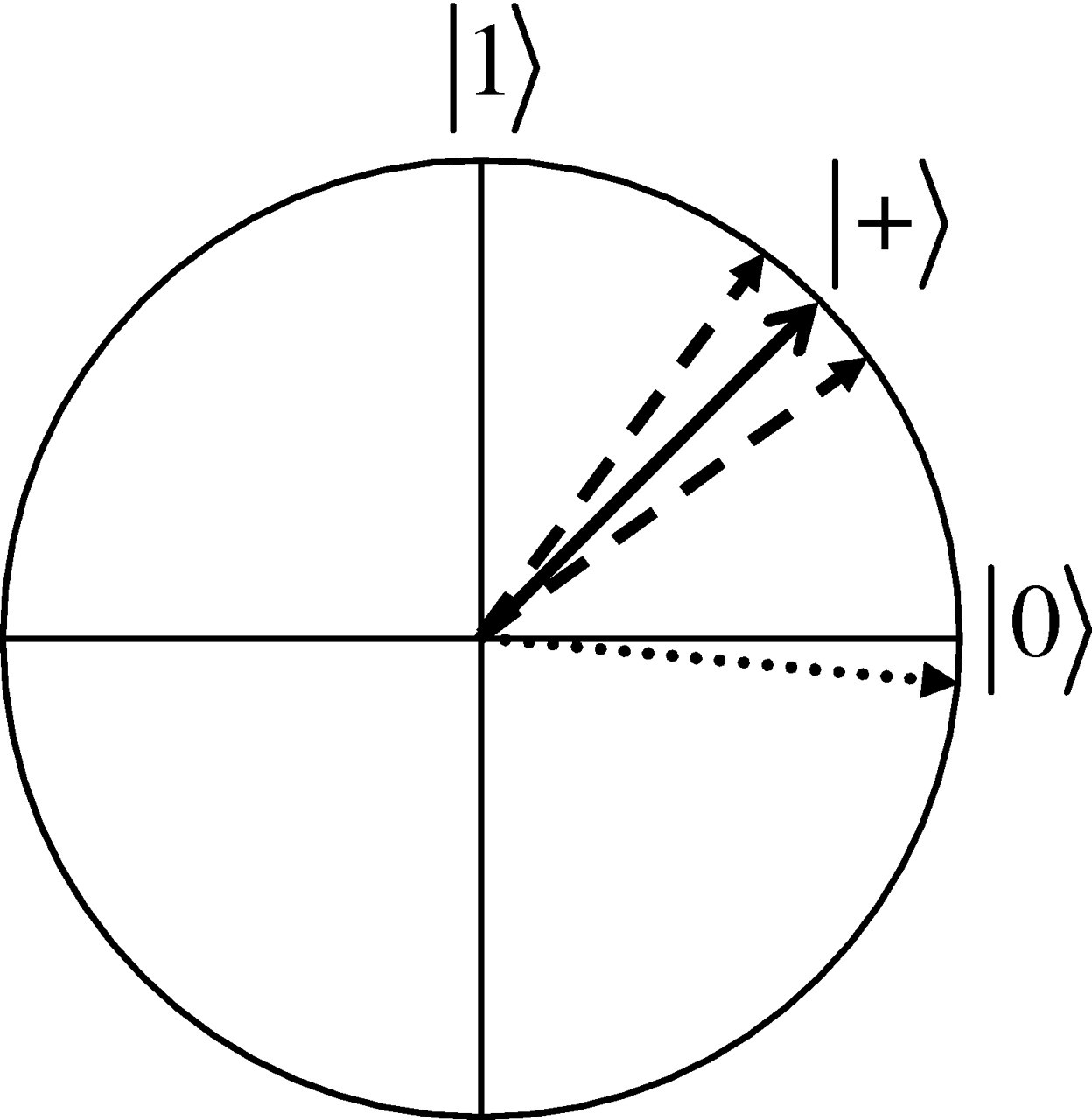
To differentiate between classical bits, in the picture from above a new notation was introduced - \(\ket{\cdot}\) - called "ket", which denotes a special kind of column vector which represents a quantum state. Also, two special cases corresponding to the classical bits \(0\) and \(1\) can be distinguished as:
\[\require{braket} \ket{0} = \col{1 \\ 0}; \quad \ket{1} = \col{0 \\ 1} \]Using this, any quantum states can be represented as a linear combination of \(\ket{0}\) and \(\ket{1}\):
\[ \col{a \\ b} = a \col{1 \\ 0} + b\col{0 \\ 1} = a \ket{0} + b \ket{1} \]This work is licensed under a Creative Commons Attribution 4.0 International License, and it can be cited as: https://zackyzz.github.io/quantum.